Grouped summarization in pandas

Grouped summarization in pandas#

# initialization
import numpy as np
import pandas as pd
import matplotlib.pyplot as plt

The .groupby() method of pandas DataFrame#

Sometimes your data can be partitioned into multiple subsets, and it would be useful to obtain summary statistics on each subset. As an example, we will use the fish length and weight data taken from Alaskan shore between 1997-2006. More information about the source data can be found on https://lod.bco-dmo.org/id/dataset/3332, and the simplified data we use can be found as the csv file here.

fish = pd.read_csv("data/secm_fish_size.csv", na_values=["nd"])
display(fish)

	date	time_local	haul_id	fish_id	lat	lon	locality	species	name_common	length	weight
0	1997-5-20	9:40	1001	6	58.19	-134.20	Taku_Inlet	Platichthys_stellatus	Starry_flounder	347.0	500.0
1	1997-5-20	9:40	1001	7	58.19	-134.20	Taku_Inlet	Platichthys_stellatus	Starry_flounder	341.0	430.0
2	1997-5-20	9:40	1001	8	58.19	-134.20	Taku_Inlet	Platichthys_stellatus	Starry_flounder	339.0	459.0
3	1997-5-20	9:40	1001	9	58.19	-134.20	Taku_Inlet	Platichthys_stellatus	Starry_flounder	337.0	398.0
4	1997-5-20	9:40	1001	10	58.19	-134.20	Taku_Inlet	Platichthys_stellatus	Starry_flounder	309.0	325.0
...	...	...	...	...	...	...	...	...	...	...	...
1723	2006-7-30	9:5	10085	17	58.10	-135.02	Upper_Chatham	Oncorhynchus_tshawytscha	Chinook_Imm.	472.0	1375.0
1724	2006-7-31	7:40	10088	27	58.22	-135.53	Icy_Strait	Oncorhynchus_tshawytscha	Chinook_Imm.	442.0	1400.0
1725	2006-7-31	10:30	10090	34	58.25	-135.44	Icy_Strait	Oncorhynchus_tshawytscha	Chinook_Imm.	563.0	2300.0
1726	2006-7-31	10:30	10090	35	58.25	-135.44	Icy_Strait	Oncorhynchus_tshawytscha	Chinook_Imm.	459.0	1150.0
1727	2006-7-31	12:0	10091	75	58.27	-135.40	Icy_Strait	Oncorhynchus_kisutch	Coho_Adult	585.0	2250.0

1728 rows × 11 columns

fish.info()

<class 'pandas.core.frame.DataFrame'>
RangeIndex: 1728 entries, 0 to 1727
Data columns (total 11 columns):
 #   Column       Non-Null Count  Dtype  
---  ------       --------------  -----  
 0   date         1728 non-null   object 
 1   time_local   1728 non-null   object 
 2   haul_id      1728 non-null   int64  
 3   fish_id      1728 non-null   int64  
 4   lat          1728 non-null   float64
 5   lon          1728 non-null   float64
 6   locality     1728 non-null   object 
 7   species      1728 non-null   object 
 8   name_common  1728 non-null   object 
 9   length       1724 non-null   float64
 10  weight       1683 non-null   float64
dtypes: float64(4), int64(2), object(5)
memory usage: 148.6+ KB

If you inspect the dataset, you will see that many fish species show up many, many times. It may be useful to find the average length of each species of fish from this dataset. To do so, we need to split the dataset by species, apply the summarization, then combine the result.

Luckily, pandas has a built-in .groupby() method to help with this split-apply-combine pipeline. The .groupby() method will create the split and perform the combination. We just have to supply the function to apply via method chaining. In our case. the summarization function is .mean(), so we do:

fish_grp_mean = fish.loc[:, ["species", "length", "weight"]].groupby("species").mean()
display(fish_grp_mean)

	length	weight
species
Anarrhichthys_ocellatus	587.000000	1130.000000
Anoplopoma_fimbria	320.172043	386.913978
Brama_japonica	351.857143	1057.692308
Clupea_pallasi	208.000000	145.000000
Gadus_macrocephalus	308.700000	229.000000
Merluccius_productus	492.500000	825.000000
Oncorhynchus_gorbuscha	498.364341	1596.613546
Oncorhynchus_keta	656.794118	3531.323529
Oncorhynchus_kisutch	599.404040	3022.421053
Oncorhynchus_nerka	613.909091	2913.636364
Oncorhynchus_tshawytscha	395.789969	1025.838095
Platichthys_stellatus	334.764706	477.176471
Sebastes_ciliatus	280.000000	350.000000
Sebastes_melanops	495.875000	2371.250000
Squalus_acanthias	657.000000	1781.518692
Theragra_chalcogramma	405.115789	516.202899
Trichodon_trichodon	171.838710	86.580645

Notice that the variable used for grouping (species) is now the index of the DataFrame. Again, we can turn the index back to a regular column via .reset_index()

fish_grp_mean = fish_grp_mean.reset_index()
fish_grp_mean

	species	length	weight
0	Anarrhichthys_ocellatus	587.000000	1130.000000
1	Anoplopoma_fimbria	320.172043	386.913978
2	Brama_japonica	351.857143	1057.692308
3	Clupea_pallasi	208.000000	145.000000
4	Gadus_macrocephalus	308.700000	229.000000
5	Merluccius_productus	492.500000	825.000000
6	Oncorhynchus_gorbuscha	498.364341	1596.613546
7	Oncorhynchus_keta	656.794118	3531.323529
8	Oncorhynchus_kisutch	599.404040	3022.421053
9	Oncorhynchus_nerka	613.909091	2913.636364
10	Oncorhynchus_tshawytscha	395.789969	1025.838095
11	Platichthys_stellatus	334.764706	477.176471
12	Sebastes_ciliatus	280.000000	350.000000
13	Sebastes_melanops	495.875000	2371.250000
14	Squalus_acanthias	657.000000	1781.518692
15	Theragra_chalcogramma	405.115789	516.202899
16	Trichodon_trichodon	171.838710	86.580645

In addition to grouped mean, the following functions are available for grouped summarization:

.count(): count the number of non-NA values in each group
.max(): Compute the maximum value in each group
.min(): Compute the minimum value in each group
.mean(): Compute the mean of each group
.median(): Compute the median of each group
.nunique(): Compute the number of unique values in each group
.quantile(): Compute a given quantile of the values in each group
.sem(): Compute the standard error of the mean of the values in each group
.std(): Compute the standard deviation of the values in each group
.var(): Compute the variance of the values in each group

Recall in week 4 we talked about the concept of standard error, which is a measure of the uncertainty in the mean. To compute the standard error, we use the .sem() method after the .groupby()

fish_grp_sem = fish.loc[
    :, ["species", "length", "weight"]
].groupby("species").sem().reset_index()

display(fish_grp_sem)

	species	length	weight
0	Anarrhichthys_ocellatus	NaN	NaN
1	Anoplopoma_fimbria	5.672692	16.722263
2	Brama_japonica	6.237830	43.796643
3	Clupea_pallasi	NaN	NaN
4	Gadus_macrocephalus	5.166237	16.512621
5	Merluccius_productus	77.500000	225.000000
6	Oncorhynchus_gorbuscha	2.567097	35.408346
7	Oncorhynchus_keta	9.004256	152.740822
8	Oncorhynchus_kisutch	13.365375	158.806295
9	Oncorhynchus_nerka	29.958291	315.514796
10	Oncorhynchus_tshawytscha	6.158532	104.286037
11	Platichthys_stellatus	12.529239	64.601564
12	Sebastes_ciliatus	NaN	NaN
13	Sebastes_melanops	30.070416	350.924481
14	Squalus_acanthias	7.639284	71.993265
15	Theragra_chalcogramma	3.817544	12.337072
16	Trichodon_trichodon	6.488882	13.225812

Note that we have a bunch of NaN in the results, which is a consequence that some species only appeared once in the dataset.

To combine the two DataFrames, we can use pd.concat() with axis=1. But because some variable names are repeated, we first have to modify those names:

fish_grp_mean.columns = ["species", "mean_length", "mean_weight"]
fish_grp_sem.columns = ["species", "stderr_length", "stderr_weight"]

fish_grp_stats = pd.concat([
    fish_grp_mean.set_index("species"), 
    fish_grp_sem.set_index("species")
], axis = 1).reset_index()

display(fish_grp_stats)

	species	mean_length	mean_weight	stderr_length	stderr_weight
0	Anarrhichthys_ocellatus	587.000000	1130.000000	NaN	NaN
1	Anoplopoma_fimbria	320.172043	386.913978	5.672692	16.722263
2	Brama_japonica	351.857143	1057.692308	6.237830	43.796643
3	Clupea_pallasi	208.000000	145.000000	NaN	NaN
4	Gadus_macrocephalus	308.700000	229.000000	5.166237	16.512621
5	Merluccius_productus	492.500000	825.000000	77.500000	225.000000
6	Oncorhynchus_gorbuscha	498.364341	1596.613546	2.567097	35.408346
7	Oncorhynchus_keta	656.794118	3531.323529	9.004256	152.740822
8	Oncorhynchus_kisutch	599.404040	3022.421053	13.365375	158.806295
9	Oncorhynchus_nerka	613.909091	2913.636364	29.958291	315.514796
10	Oncorhynchus_tshawytscha	395.789969	1025.838095	6.158532	104.286037
11	Platichthys_stellatus	334.764706	477.176471	12.529239	64.601564
12	Sebastes_ciliatus	280.000000	350.000000	NaN	NaN
13	Sebastes_melanops	495.875000	2371.250000	30.070416	350.924481
14	Squalus_acanthias	657.000000	1781.518692	7.639284	71.993265
15	Theragra_chalcogramma	405.115789	516.202899	3.817544	12.337072
16	Trichodon_trichodon	171.838710	86.580645	6.488882	13.225812

Example: climatology#

As a second example, suppose we are interested in climatology, i.e., the long term weather pattern. Our source data are weather information at the SeaTac airport and Spokane airport, from 2020 to 2024. The data is sourced from NOAA Climate Data Online, and a copy of the simplified and combined data we use can be found here.

WA_weather = pd.read_csv("data/WA_weather_2000-2024.csv", parse_dates = ["DATE"])
display(WA_weather)

	NAME	LATITUDE	LONGITUDE	ELEVATION	DATE	PRCP	TAVG	TMAX	TMIN
0	SEATTLE TACOMA AIRPORT, WA US	47.44467	-122.31442	112.5	2000-01-01	6.9	4.4	6.1	2.8
1	SEATTLE TACOMA AIRPORT, WA US	47.44467	-122.31442	112.5	2000-01-02	0.0	-3.9	7.2	2.8
2	SEATTLE TACOMA AIRPORT, WA US	47.44467	-122.31442	112.5	2000-01-03	7.1	5.6	8.3	2.2
3	SEATTLE TACOMA AIRPORT, WA US	47.44467	-122.31442	112.5	2000-01-04	7.6	7.8	10.0	5.6
4	SEATTLE TACOMA AIRPORT, WA US	47.44467	-122.31442	112.5	2000-01-05	0.0	5.0	6.7	2.8
...	...	...	...	...	...	...	...	...	...
18259	SPOKANE INTERNATIONAL AIRPORT, WA US	47.62168	-117.52796	717.7	2024-12-27	0.8	2.7	4.4	0.6
18260	SPOKANE INTERNATIONAL AIRPORT, WA US	47.62168	-117.52796	717.7	2024-12-28	4.3	4.4	7.2	3.3
18261	SPOKANE INTERNATIONAL AIRPORT, WA US	47.62168	-117.52796	717.7	2024-12-29	15.2	3.7	3.9	0.6
18262	SPOKANE INTERNATIONAL AIRPORT, WA US	47.62168	-117.52796	717.7	2024-12-30	8.9	1.1	2.8	-1.6
18263	SPOKANE INTERNATIONAL AIRPORT, WA US	47.62168	-117.52796	717.7	2024-12-31	0.3	0.1	1.1	-1.6

18264 rows × 9 columns

WA_weather.info()

<class 'pandas.core.frame.DataFrame'>
RangeIndex: 18264 entries, 0 to 18263
Data columns (total 9 columns):
 #   Column     Non-Null Count  Dtype         
---  ------     --------------  -----         
 0   NAME       18264 non-null  object        
 1   LATITUDE   18264 non-null  float64       
 2   LONGITUDE  18264 non-null  float64       
 3   ELEVATION  18264 non-null  float64       
 4   DATE       18264 non-null  datetime64[ns]
 5   PRCP       18259 non-null  float64       
 6   TAVG       12654 non-null  float64       
 7   TMAX       18264 non-null  float64       
 8   TMIN       18263 non-null  float64       
dtypes: datetime64[ns](1), float64(7), object(1)
memory usage: 1.3+ MB

To proceed, we extract the day of year from the timestamp, which we’ll use as our group-by variable:

WA_weather["day_of_year"] = WA_weather["DATE"].dt.dayofyear

Now we can perform the group-by and compute the mean and standard error. Note that since we have two locations that we want to analyze separately, we need to group by both NAME and day_of_year:

WA_weather_mean = WA_weather.groupby(
    ["NAME", "day_of_year"]
).mean(numeric_only=True).reset_index()

WA_weather_sem = WA_weather.groupby(
    ["NAME", "day_of_year"]
).sem(numeric_only=True).reset_index()

WA_weather_mean

	NAME	day_of_year	LATITUDE	LONGITUDE	ELEVATION	PRCP	TAVG	TMAX	TMIN
0	SEATTLE TACOMA AIRPORT, WA US	1	47.44467	-122.31442	112.5	4.688000	4.276471	7.736000	1.844000
1	SEATTLE TACOMA AIRPORT, WA US	2	47.44467	-122.31442	112.5	7.264000	4.029412	7.820000	1.928000
2	SEATTLE TACOMA AIRPORT, WA US	3	47.44467	-122.31442	112.5	4.600000	4.988235	8.104000	2.112000
3	SEATTLE TACOMA AIRPORT, WA US	4	47.44467	-122.31442	112.5	5.864000	5.229412	7.980000	2.720000
4	SEATTLE TACOMA AIRPORT, WA US	5	47.44467	-122.31442	112.5	5.540000	5.147059	8.076000	3.072000
...	...	...	...	...	...	...	...	...	...
727	SPOKANE INTERNATIONAL AIRPORT, WA US	362	47.62168	-117.52796	717.7	2.372000	-2.082353	0.684000	-3.824000
728	SPOKANE INTERNATIONAL AIRPORT, WA US	363	47.62168	-117.52796	717.7	2.172000	-2.535294	0.744000	-4.868000
729	SPOKANE INTERNATIONAL AIRPORT, WA US	364	47.62168	-117.52796	717.7	2.672000	-2.600000	-0.364000	-5.756000
730	SPOKANE INTERNATIONAL AIRPORT, WA US	365	47.62168	-117.52796	717.7	2.464000	-2.952941	-0.756000	-6.404000
731	SPOKANE INTERNATIONAL AIRPORT, WA US	366	47.62168	-117.52796	717.7	0.842857	-1.320000	0.414286	-4.728571

732 rows × 9 columns

WA_weather_mean = WA_weather_mean.loc[
    :, ["NAME", "day_of_year", "PRCP", "TAVG", "TMAX", "TMIN"]
]

WA_weather_sem = WA_weather_sem.loc[
    :, ["NAME", "day_of_year", "PRCP", "TAVG", "TMAX", "TMIN"]
]

WA_weather_mean.columns = [
    "NAME", "day_of_year", "PRCP_mean", "TAVG_mean", "TMAX_mean", "TMIN_mean"
]

WA_weather_sem.columns = [
    "NAME", "day_of_year", "PRCP_sem", "TAVG_sem", "TMAX_sem", "TMIN_sem"
]

WA_weather_stat = pd.concat([
    WA_weather_mean.set_index(["NAME", "day_of_year"]),
    WA_weather_sem.set_index(["NAME", "day_of_year"])
], axis = 1).reset_index()    

display(WA_weather_stat)

	NAME	day_of_year	PRCP_mean	TAVG_mean	TMAX_mean	TMIN_mean	PRCP_sem	TAVG_sem	TMAX_sem	TMIN_sem
0	SEATTLE TACOMA AIRPORT, WA US	1	4.688000	4.276471	7.736000	1.844000	1.379690	0.843423	0.635082	0.761732
1	SEATTLE TACOMA AIRPORT, WA US	2	7.264000	4.029412	7.820000	1.928000	2.506318	0.945335	0.659722	0.685845
2	SEATTLE TACOMA AIRPORT, WA US	3	4.600000	4.988235	8.104000	2.112000	1.353255	0.837006	0.721376	0.732719
3	SEATTLE TACOMA AIRPORT, WA US	4	5.864000	5.229412	7.980000	2.720000	1.405938	1.042895	0.787274	0.800854
4	SEATTLE TACOMA AIRPORT, WA US	5	5.540000	5.147059	8.076000	3.072000	1.581086	1.052522	0.750628	0.855015
...	...	...	...	...	...	...	...	...	...	...
727	SPOKANE INTERNATIONAL AIRPORT, WA US	362	2.372000	-2.082353	0.684000	-3.824000	0.652394	0.866460	0.768346	0.818235
728	SPOKANE INTERNATIONAL AIRPORT, WA US	363	2.172000	-2.535294	0.744000	-4.868000	0.935566	0.942460	0.770348	0.887087
729	SPOKANE INTERNATIONAL AIRPORT, WA US	364	2.672000	-2.600000	-0.364000	-5.756000	0.914577	1.119381	0.786318	0.953748
730	SPOKANE INTERNATIONAL AIRPORT, WA US	365	2.464000	-2.952941	-0.756000	-6.404000	0.981884	0.988579	0.826803	1.228257
731	SPOKANE INTERNATIONAL AIRPORT, WA US	366	0.842857	-1.320000	0.414286	-4.728571	0.425305	1.413294	0.742399	1.844776

732 rows × 10 columns

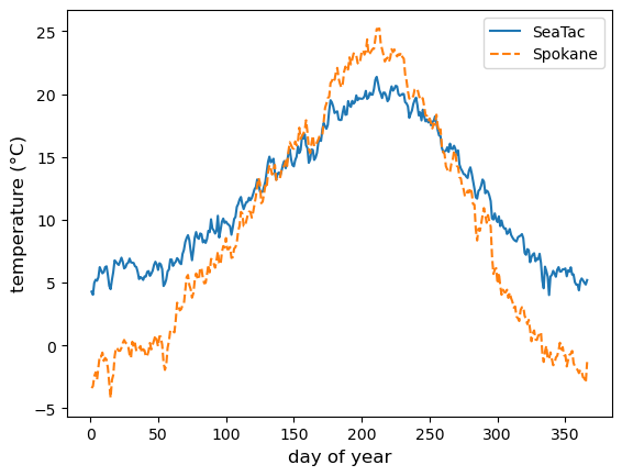
Now we can visualize the climatology of average temperature with a plot:

spokane_stat = WA_weather_stat.loc[WA_weather_stat["NAME"] == "SPOKANE INTERNATIONAL AIRPORT, WA US"]
seatac_stat = WA_weather_stat.loc[WA_weather_stat["NAME"] == "SEATTLE TACOMA AIRPORT, WA US"]

fig = plt.figure()
ax = fig.add_subplot()

ax.plot(seatac_stat["day_of_year"], seatac_stat["TAVG_mean"], ls = "-", label="SeaTac")
ax.plot(spokane_stat["day_of_year"], spokane_stat["TAVG_mean"], ls = "--", label="Spokane")

ax.set_xlabel("day of year", fontsize=12)
ax.set_ylabel("temperature (°C)", fontsize=12)

ax.legend()

plt.show(fig)

../_images/83a924d5b6cb2afa251be67c9f17547b3afb900bfb3b035e405fa992ede453ec.png

Grouped summarization in pandas

Contents

Grouped summarization in pandas#

The .groupby() method of pandas DataFrame#

Example: climatology#