Introduction to cartopy

Introduction to cartopy#

# initialization
import numpy as np
import pandas as pd
import xarray as xr
import matplotlib.pyplot as plt

Prelude: the Earth is round, but the map is flat#

Due to the fundamental fact that the Earth is round, it is impossible to represent all of areas, lengths, and angles faithfully on a flat sheet. Therefore, all maps are distorted in one way or another. However, different projection of the curved Earth surface onto flat 2-dimensional sheets may be more or less useful in a given situation.

Up to this point, we have been treating longitude and latitude as ordinary x- and y- axis. As a result, when we plot both longitude (as x-axis) and latitude (as y-axis), we have essentially been using the plate carrée map projection, which distorts areas and lengths as we move away from the equator.

In matplotlib, there is no easy way to switch to a different projection. However, the third-party cartopy module can be used to extend matplotlib, thus allowing us to specify data in the plate carrée coordinates but present them under a different projection. In addition, cartopy also comes bundled with information about geographical features, which can be conveniently included in plots.

Map projections in cartopy#

Instead of importing the entire cartopy package, we import two submodules from it:

import cartopy.crs as ccrs
import cartopy.feature as cfeature

(Note that crs is short for coordinate reference system)

The ccrs submodule provide tools for map projection, while cfeature let us include geographical features in our plots.

A cartopy plot is not much different from a standard matplotlib plot, except that: (1) when Axes instances are created, we need to supply one of the crs implemented by cartopy in the projection argument; (2) when we add data via .polormesh(), .contour(), etc., we need to supply the source crs using the transform argument.

To illustrate how cartopy works, we display the world’s coastline using the .coastlines() method, available to all cartopy-augmented Axes instances, for the usual plate carrée projection:

fig = plt.figure(figsize=(5, 3))
ax = fig.add_subplot(projection=ccrs.PlateCarree())

ax.coastlines()

plt.show(fig)

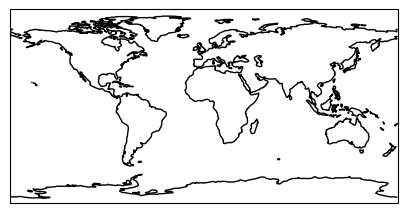
../_images/dda7c45d708482b5a00593f9d0cf35173d2714b63d5d2771ea1b19bd28d1b6ba.png

Again, note that the above code block is similar to how typical matplotlib plot is created thus far except for the projection=ccrs.PlateCarree() argument in .add_subplot(), and the ax.coastlines() line that generates the coastlines in the plot.

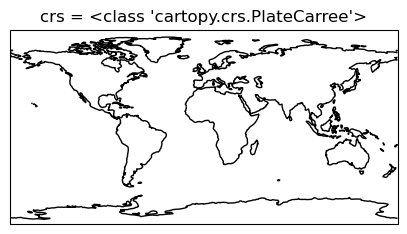
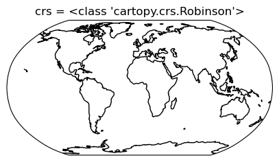
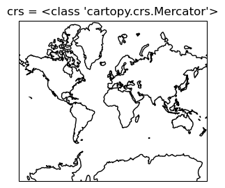
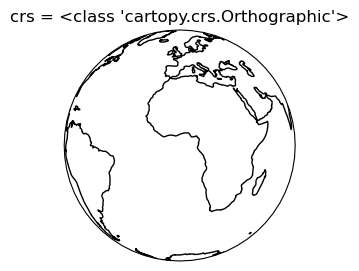
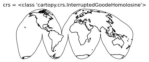
Next, we show the same coastlines in a few different map projections:

projections = [
    ccrs.PlateCarree(),
    ccrs.Robinson(),
    ccrs.Mercator(),
    ccrs.Orthographic(),
    ccrs.InterruptedGoodeHomolosine()
]

for proj in projections:
    fig = plt.figure(figsize=(5, 3))
    ax = fig.add_subplot(projection=proj)
    ax.coastlines()
    ax.set_title("crs = " + str(type(proj)))
    plt.show(fig)

../_images/a5e42e3adc88dffebbeae950787c819fee6e1093c41f61fd976bf4609092f817.png

../_images/0aef20c99f3abf5baa7c82beac8363078c86c677c86af6d08e8bf7e6e3fd72a3.png

../_images/48d11d5027130f02414935e2b747e9201dd18d40f9df3b47be4bdccc04c1c04c.png

../_images/6f2a00a3d9eb57718a32bff1a6bbb2c55fee13b0ab0ded50635c9667aff1d5b8.png

../_images/8ade67e6d144dcdb6b78b0b8915d7647b49fa38bf98884373f20ebccdb228d7c.png

For a full list of supported map projection, see https://scitools.org.uk/cartopy/docs/v0.15/crs/projections.html. In addition, a good resource for more information about various map projections is provided by ArcGIS and can be found here (unfortunately, the ArcGIS projection name does not always match that of cartopy)

If you are plotting global data, the Robinson projection may serve as a good default.

Plotting global ocean data#

Next we consider including actual data in our plot. For our examples we will be using the data from the World Ocean Atlas 2023. A copy of the data we use can be found here. We will plot the ocean surface oxygen concentration. We first load the data (note: the WOA dataset has an unusual encoding for time, so to avoid problems we set decode_times=False in xr.open_dataset()):

The variable we want to plot is o_mn and we are interested only in data at depth = 0 m, hence we subset as follows:

oxygen = woa23_O["o_mn"].sel(depth=0).squeeze().values
oxygen.shape

(36, 72)

We also extract the internal numpy array for the lat and lon coordinates:

lat = woa23_O.coords["lat"].values
lon = woa23_O.coords["lon"].values

Now we use matplotlib + cartopy to create our plot:

fig = plt.figure(figsize=(9, 4))
ax = fig.add_subplot(projection=ccrs.Robinson())

im = ax.pcolormesh(lon, lat, oxygen, transform=ccrs.PlateCarree())
cb = fig.colorbar(im)

cb.set_label("Oxygen (μmol/kg)")

ax.coastlines()

plt.show(fig)

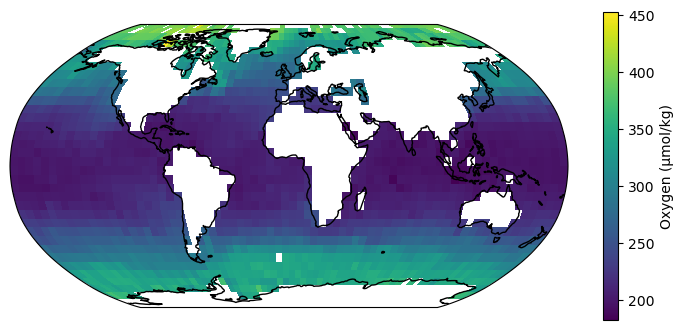
../_images/d7a6e5364516dc4e45ca3b086f493295a89f0855803e9dadd8f8eafd49600ed7.png

(The pixelation is a result of the low resolution of the dataset we picked. There is also a larger, 1° resolution dataset available from WOA)

Again, note that our block of code is similar to that of a regular matplotlib plot, except for the projection=ccrs.Robinson() argument in .add_subplot() and the transform=ccrs.PlateCarree() argument in .pcolormesh()

Introduction to cartopy

Contents

Introduction to cartopy#

Prelude: the Earth is round, but the map is flat#

Map projections in cartopy#

Plotting global ocean data#