More on cartopy#
# initialization
import numpy as np
import pandas as pd
import xarray as xr
import matplotlib.pyplot as plt
import cartopy.crs as ccrs
import cartopy.feature as cfeature
Adding geographical features#
In addition to ax.coastline(), cartopy provides a number of built-in geographical features that can be included in a plot using ax.add_feature(). The included features are:
cfeatures.BORDERS: country boundaries.cfeatures.STATES: state and province boundaries.cfeature.COASTLINE: coastline, including major islands.cfeature.LAKES: natural and artificial lakes.cfeatures.LAND: land polygons, including major islands.cfeature.OCEAN: ocean polygons.cfature.RIVERS: single-line drainages, including lake centerlines.
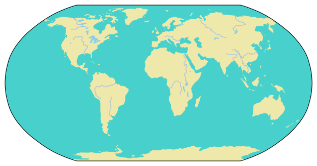
As an example, here is a cartopy plot with land, ocean, lakes, and rivers included:
fig = plt.figure(figsize=(9, 4))
ax = fig.add_subplot(projection=ccrs.Robinson())

ax.add_feature(cfeature.LAND, color="palegoldenrod")
ax.add_feature(cfeature.OCEAN, color="mediumturquoise")
ax.add_feature(cfeature.LAKES, color="skyblue")
ax.add_feature(cfeature.RIVERS, edgecolor="lightsteelblue")

plt.show(fig)
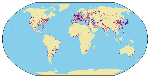
In addition, cartopy also supports adding features available from Natural Earth using the cfeature.NaturalEarthFeature() function. Here is an example of adding urban areas at the 1:50m scale (note that using the finest 1:10m scale can lead to substantial download and rendering time increases):
urban = cfeature.NaturalEarthFeature(
    category = "cultural", name = "urban_areas", scale='50m'
)

fig = plt.figure(figsize=(9, 4))
ax = fig.add_subplot(projection=ccrs.Robinson())

ax.add_feature(cfeature.LAND, color="palegoldenrod")
ax.add_feature(cfeature.OCEAN, color="skyblue")
ax.add_feature(urban, color="purple")

plt.show(fig)
Adding gridlines#
The maps we have produced so far are good for making an overall impression but are not especially useful for quantitative purposes, since there is no gridlines to help identify the coordinates of locations. To add gridlines, we can use the .gridlines() method of the cartopy-augmented Axes instance. For example:
urban = cfeature.NaturalEarthFeature(
    category = "cultural", name = "urban_areas", scale='50m'
)

fig = plt.figure(figsize=(9, 4))
ax = fig.add_subplot(projection=ccrs.Robinson())

ax.add_feature(cfeature.LAND, color="palegoldenrod")
ax.add_feature(cfeature.OCEAN, color="skyblue")
ax.add_feature(urban, color="purple")

ax.gridlines(
    crs=ccrs.PlateCarree(), draw_labels=True,
    linewidth=1, color='gray', alpha=0.5, linestyle='--'
)

plt.show(fig)
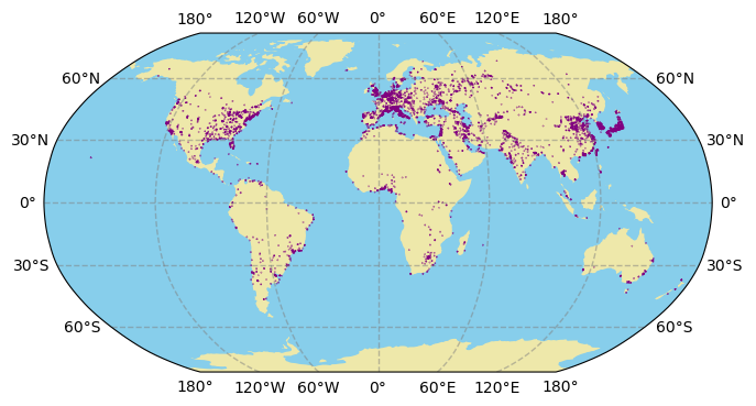
To further customize the gridlines, we assign the output of ax.gridlines() to a variable and modify its attributes. For example:
import matplotlib.ticker as mticker
from cartopy.mpl.gridliner import LONGITUDE_FORMATTER, LATITUDE_FORMATTER
urban = cfeature.NaturalEarthFeature(
category = "cultural", name = "urban_areas", scale='50m'
)
fig = plt.figure(figsize=(9, 4))
ax = fig.add_subplot(projection=ccrs.Robinson())
ax.add_feature(cfeature.LAND, color="palegoldenrod")
ax.add_feature(cfeature.OCEAN, color="skyblue")
ax.add_feature(urban, color="purple")
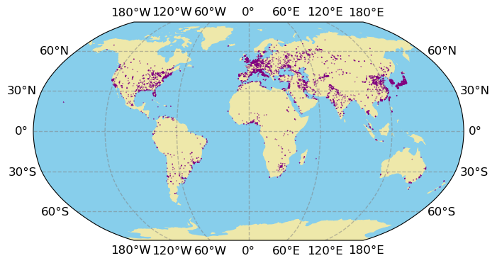
gl = ax.gridlines(
crs=ccrs.PlateCarree(), draw_labels=True,
linewidth=1, color='gray', alpha=0.5, linestyle='--'
)
gl.xlocator = mticker.FixedLocator(np.arange(-180, 181, 60))
gl.ylocator = mticker.FixedLocator(np.arange(-60, 61, 30))
gl.xformatter = LONGITUDE_FORMATTER
gl.yformatter = LATITUDE_FORMATTER
gl.xlabel_style = {'size': 12}
gl.ylabel_style = {'size': 12}
plt.show(fig)
Notice that LONGITUDE_FORMATTER and LATITUDE_FORMATTER comes from the cartopy.mpl.gridliner submodule, and the FixedLocator() function comes from the matplotlib.ticker submodule
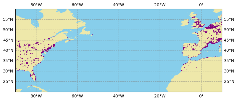
Limiting the extent of the map#
Sometimes you’ll be interested in a smaller geographical region and want the convenience of using available geographical features from cartopy. To limit the range of latitude and longitude in a cartopy plot, use the .set_extent() method of the cartopy-augmented Axes instance. For example, suppose we’re interested in the north Atlantic ocean, we may do:
urban = cfeature.NaturalEarthFeature(
    category = "cultural", name = "urban_areas", scale='50m'
)

fig = plt.figure(figsize=(9, 4))
ax = fig.add_subplot(projection=ccrs.PlateCarree())

# format: [min_lon, max_lon, min_lat, max_lat]
ax.set_extent([-90, 10, 20, 60], crs=ccrs.PlateCarree())

ax.add_feature(cfeature.LAND, color="palegoldenrod")
ax.add_feature(cfeature.OCEAN, color="skyblue")
ax.add_feature(urban, color="purple")

ax.gridlines(
    crs=ccrs.PlateCarree(), draw_labels=True,
    linewidth=1, color='gray', alpha=0.5, linestyle='--'
)

plt.show(fig)